In this two part blog post I go over my solution for the Avito challenge competition on Kaggle. It was a pretty interesting competition since it forced me to use many techniques across different fields in Machine Learning like Natural Language Processing and Computer vision. The solution is divided into two parts:

• Part 1 focuses on explaining the problem and some of the feature engineering used
• Part 2 looks at the different models tried and also the stacking methodology

The Problem:

Link to Kaggle page

Avito is a russian online advertisement company. For people living in Canada, think Kijiji but russian. People want to sell items or services to others and will therefore post online a description of the item, a picture and a price. The task is to predict whether or not an advertisement posted will lead to a deal or not. It is important to note that Avito has a more complicated system than 1/0 for a deal, making the target variable a continuous number between 0 and 1 (leading to a regression task) rather than a binary variable. The training data given is 1.5 million ads and we have to predict 500K ads from a test set. The quality of the predictions is evaluated with root mean squared error (RMSE) which is pretty common for regression tasks.

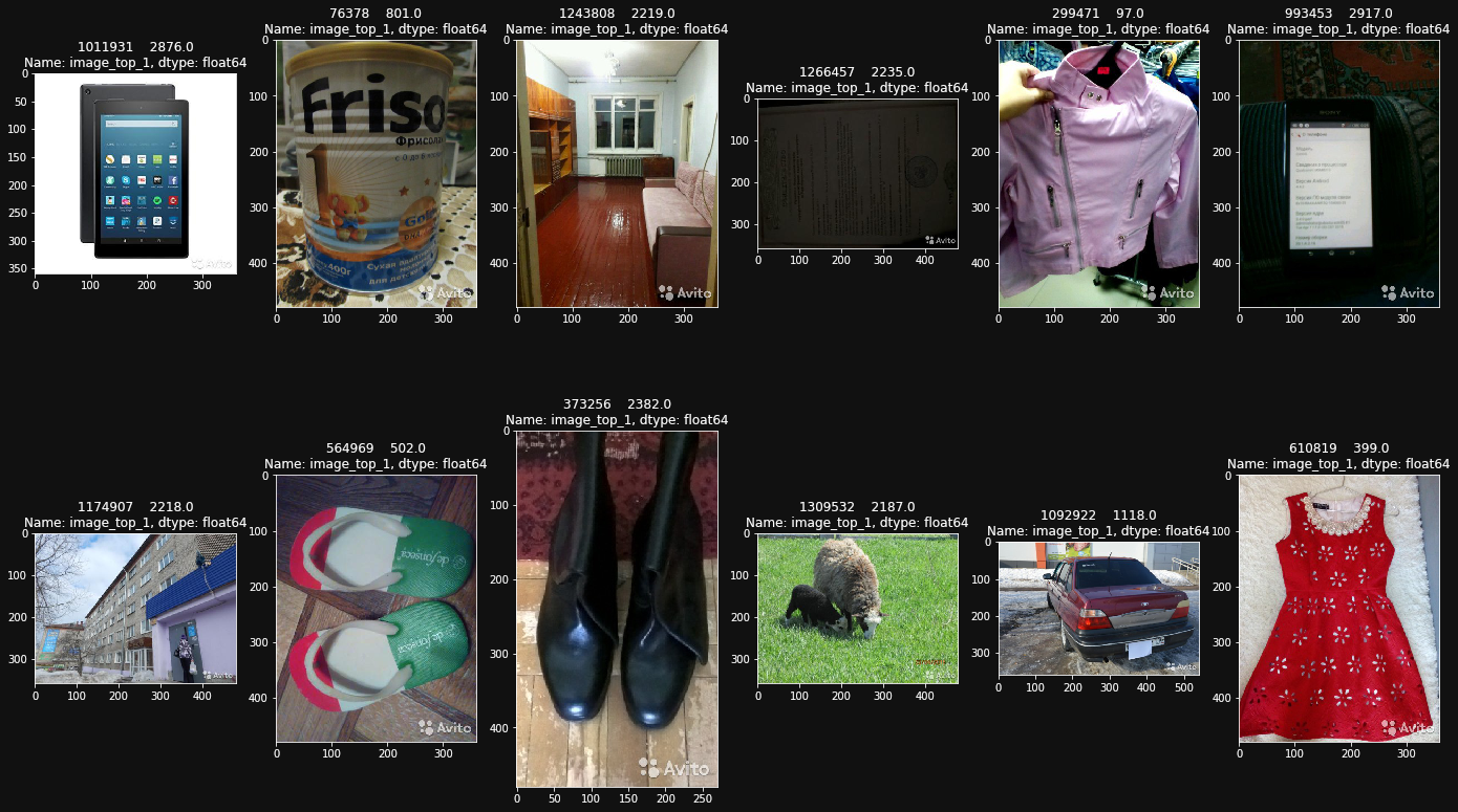Some Images in the collection

The data given to us is very rich:

• Some information about the advertisement like price, city, region, user (who posted).
• Title and Description texts.
• Image associated to the ad (maximum of 1 image per ad).
• A large dataset without the target (and which is not part of the test set either).

Note that the text is in russian, creating some additional difficulty for analysis. Here is an example :

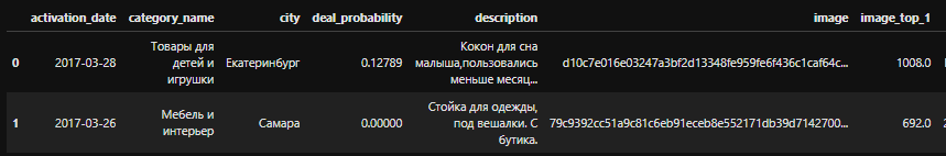An example in the dataset

Features

For exploratory data analysis I strongly suggest going over my notebook on github. See the markdown version here. It contains most of the important parts.

Missing Data
Early models showed a big importance of some variables most notably price and image_top_1. Image top 1 is assumed to be some classification of the image for an advertisement. Since I found a strong correlation with the target variable, it was deemed necessary to impute missing prices and image_top_1 with a model rather than a simple method like the mean or median. The way it was modelled was to use a recurrent neural network trained on reading the texts and predict the image_top_1 category. Here is the architecture used:

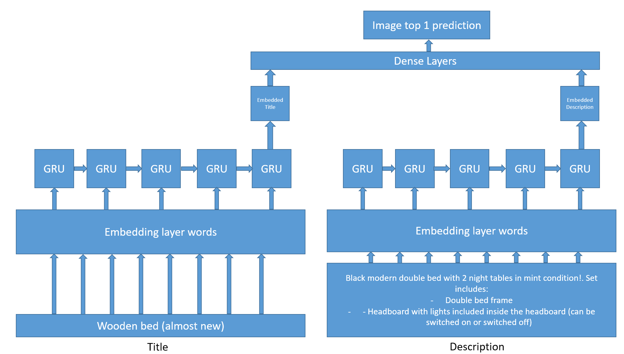RNN architecture for image_top_1 imputation

A similar idea was used for price but simply adding the city as a potential factor for determining price. You can also find the notebooks for this in the imputation subdirectory of the github repo. As you have noticed, an embedding layer for words is used. The embedding have been trained on the larger dataset that doesn’t contain the target variable. It is rich in descriptions so a simply word2vec algorithm was made on its corpus of text using gensim library. To know more about word2vec and the different ways of finding word embeddings you can view this page for example.

Text Features
Two categories of features are derived from the text data. The meta text features and features based on content. The meta text features contain things like:

• Length of the title or description
• Number of uppercase (maybe too much uppercase is detrimental)
• Ratio of length between title and description
• Ratio of unique words
• etc.

The gain in predictive power out of these features is small but it’s a gain nonetheless. For the text itself, when used in a neural network it is used as is (after tokenization) but for classical machine learning like trees we need to transform the text. A simple TF-IDF method is used for the description. Term Frequency inverse document frequency (TF-IDF) simply counts the number of occurences of each word in each texts and divides by the number of time the word appears at least one across texts. Here is an illustration:

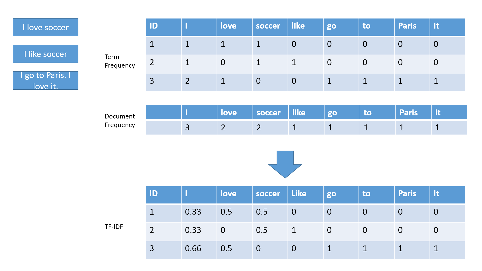TF-IDF illustration

As you can see it creates a very long vector of numbers for each document. That vector is used as a feature in a model (as will be seen in part2). It may sound like too many features due to large vocabularies (sometimes in the millions) but the vector is usually sparse (full of 0) so some algorithms are able to use that fact to have efficient ways of dealing with this long vector.

Image Features
Due to a lack of time images were dealt with in two simple ways. Similar to text, we have meta image features:

• Height, Width
• Size
• Blurness
• Brightness
• Dominant colors

These ended up helping very little.

For the images themselves, in a neural network one way to deal with it would be to build a convolutional neural net on images before concatenating with other features but this requires a lot of computing power and I lacked time. Instead a simple approach was used: using pretrained models. The Keras library offers pretrained models that perform well on an image classification task called ImageNet. The idea was to simply load them and make them predict the image class of the images. To reduce variance 3 models are used (Resnet, Inception, Exception) and the top 3 classes are considered.

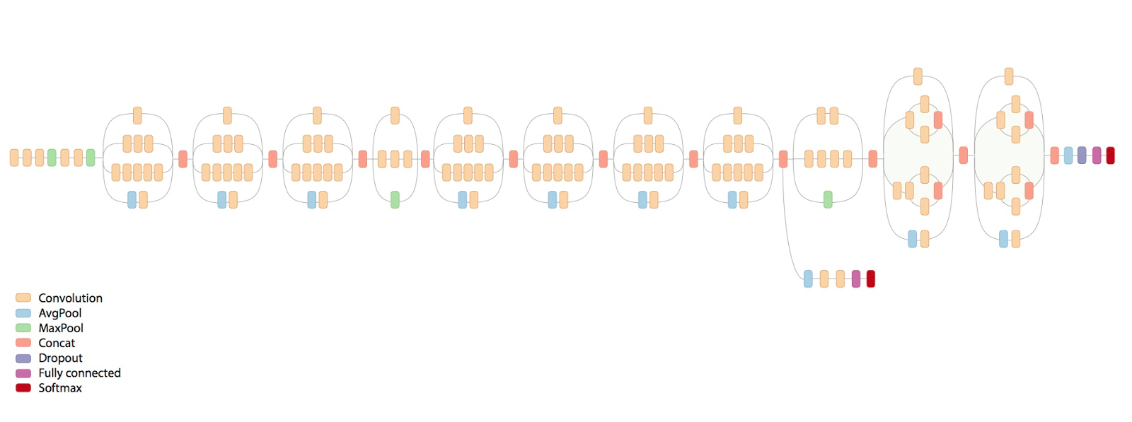Inception model Source Google AI blog

The idea is to simply predict the top 3 classes for the 3 models. This creates 9 labels per image. Then a simple term frequency of the class predicted is used to create features. At first, I tried to use the top labels directly as a categorical feature but it ended up overfitting. To mitigate the overfitting I decided to add more labels to reduce variability as I suspected the top of predictions of these models to be too imprecise to really mean something but helping the model to only learn the train set. Using 9 labels in a bag of word fashion negated the issue and helped the model a bit.

All image processes are available in the Image subdirectory of the repository.

Go to part 2