If you haven’t seen the first part please go there to have a better understanding of what is the problem and what kind of preprocessing was done on the data before the model stage: Part 1.

Models

Two kind of models were used in this competition. I will expose briefly the ideas behind each of them. First let’s get an overview:

• Neural Network
• GBDT with LightGBM
• GBDT with catboost

Neural Network

I encountered a lot of interesting insights while doing this competition. First, there is a clever way to deal with categorical variables in a neural network. I was used to believe you had to one hot encode it or find some other form of encoding. Well, it turns out there is a natural way to encode things… using embedding layers. You can read the paper here. It works similarly than for word. When the network sees a categorical value, for example ‘Rome’ in the category ‘City’, it looks into a dictionnary of vectors (the embedding layer) and then sends forward this vector of numbers to the next layer (usually other numerical features). The vectors starts with random values and then are trained. This creates a vectorized representation of the categorical values.

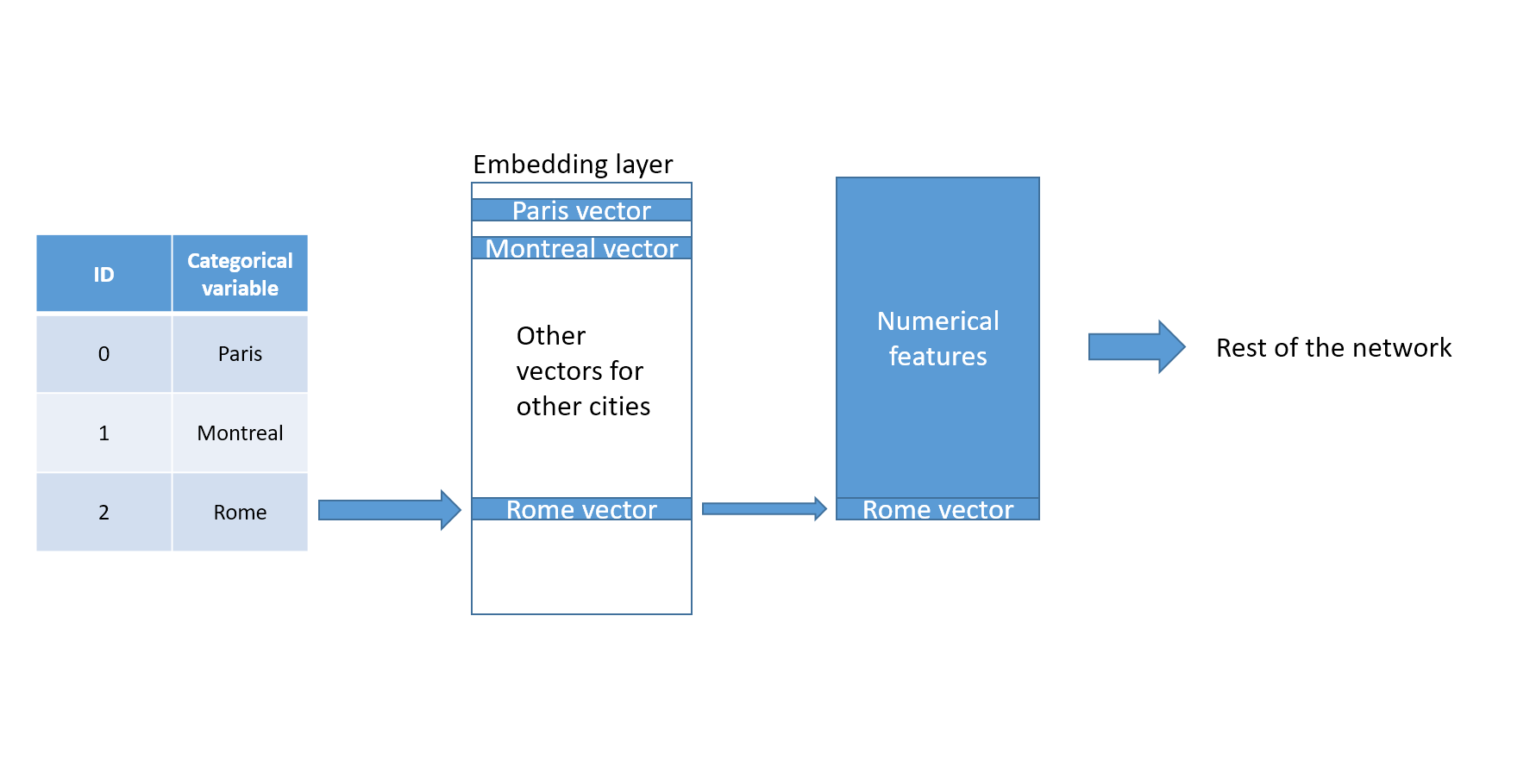
Observation with ‘Rome’ value through embedding layer

One of the advantage of that technique is that the network now has representations that can be used elsewhere. For example, we could now after training compare the vectors of Rome and Paris and see if they are close or not. This would give us an idea (for the task) what cities react in similar or dissimilar ways. The embedded layer can even be reused as a starting block for another task like when we use pretrained word embeddings.

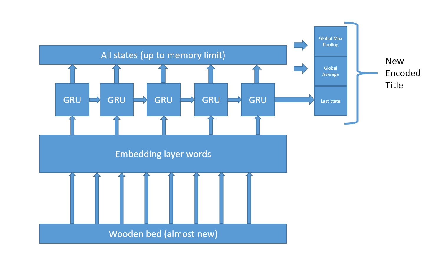
Second, when dealing with text data Jeremy Howard and Sebastian Ruder suggest in a paper to use both the last state, an average of all states and a maxpool of all state at the end of a recurrent network layer. So instead of doing this :

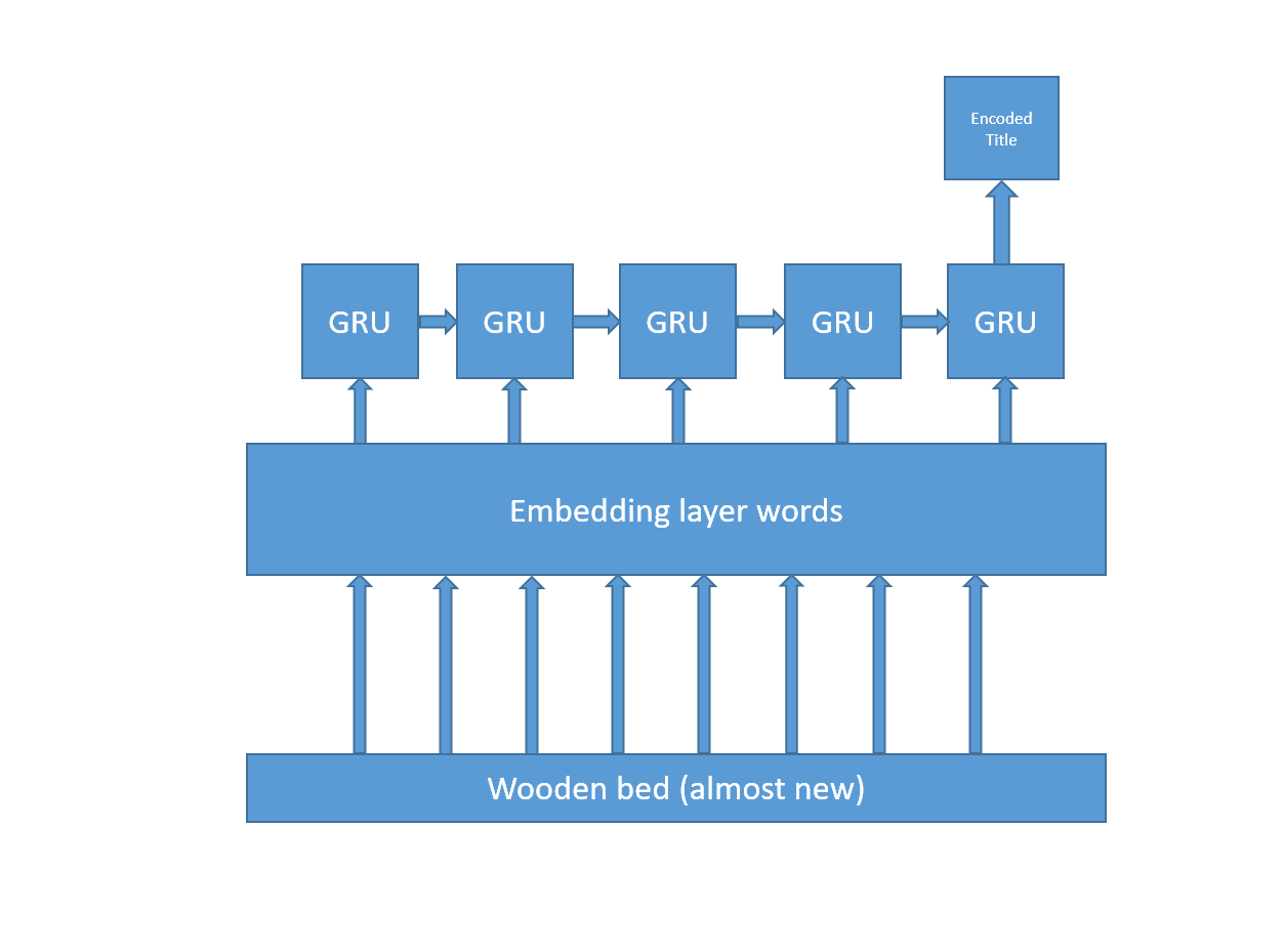
they suggest doing this :

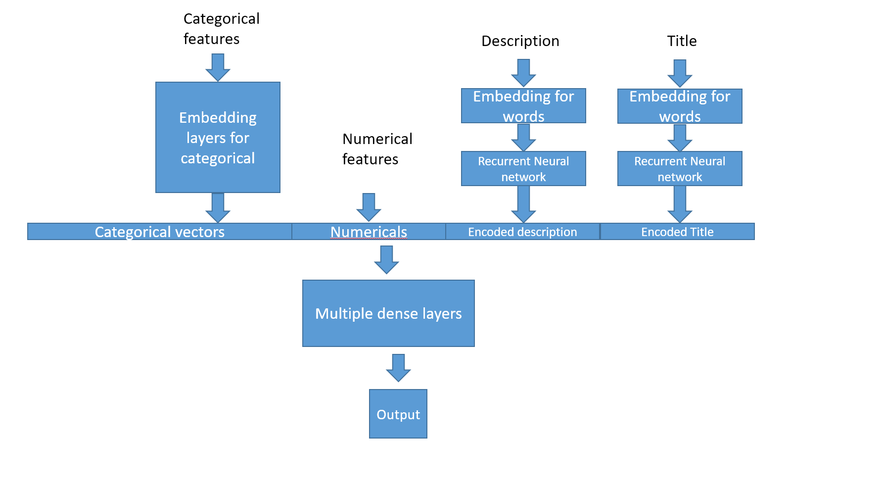
So to sum up:

• Categoricals go through an embedding layer
• Texts go first through an embedding and then through a recurrent layer to produce a numerical vector for the whole text
• Concatenate everything to the numericals
• Pass everything through fully connected layers

Here is how the final architecture looks like :

The performance were good but I had something a bit better with the lightgbm GBDT that we will see next.

GBDT models

This sub section talks about both catboost and lightgbm which are two variant of gradient boosted decision tress (GBDT). GBDT have been winning a lot of competition these past years for tabular data. I usually use them as the default algorithm just to have a good benchmark or find features importance. The logic behind GBDTs is fairly simple to understand. At every step make a new tree that tries to be good where the previous tree was weak. Then, make a prediction based on the average prediction of all trees.

GBDT algorithm mostly vary in how they make each individual trees. In our case, Catboost and LightGBM have two important differences. First, lightGBM is able to deal with sparse matrixes. This is very important in our case because like said in part 1 I use a TF-IDF matrix for the texts. Trying to use these sparse matrices in catboost would fail because the algorithm would try to make it a dense matrix and get an out of memory error. However, there is a solution to use texts in catboost. Since we have a big matrix we can simply use a dimensionality reduction procedure like singular value decomposition (SVD) to get only a few dozen of the most important components out of the sparse matrix. In a sense this is similar to encoding the text into a dense small vector.

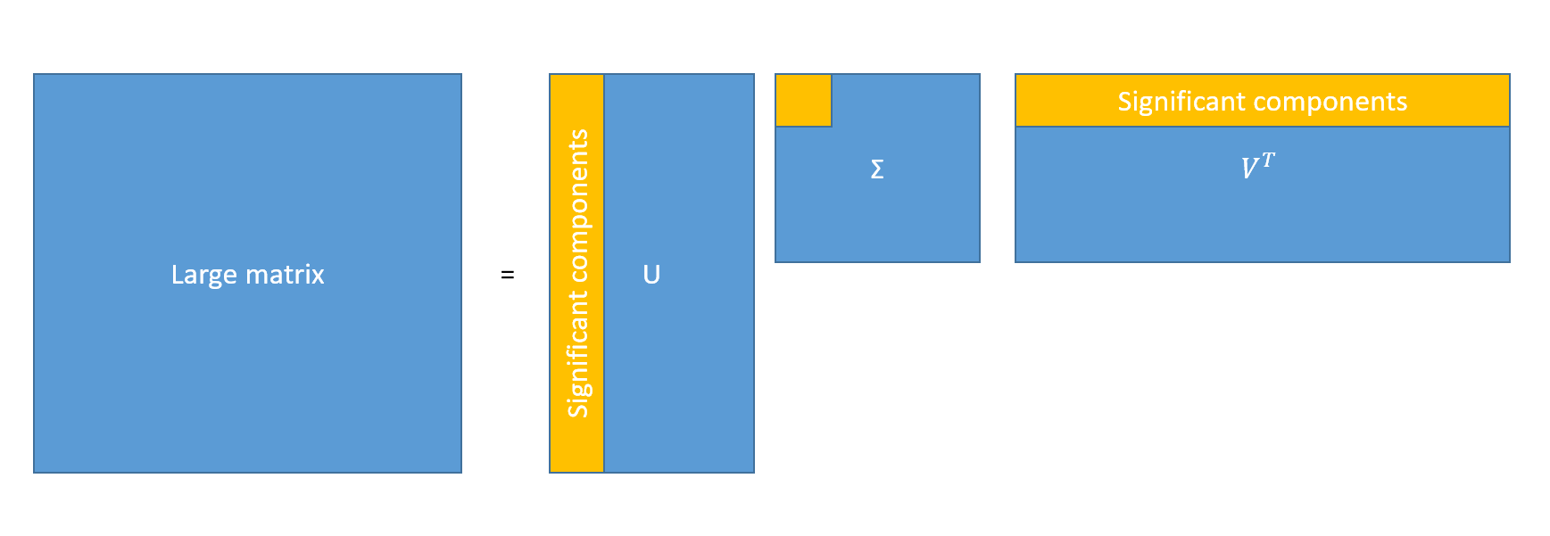Singular value decomposition

Catboost specializes in dealing with categorical data. For a gradient boosted method, it has to deal with numerical values and therefore must use some calculations for categoricals to be able to make branches in the trees based on these features. Catboost uses a costly but less biased algorithm to make those calculations. In simple words it first shuffle the data and then uses a cummulative mean of the target variable to learn if a categorical feature is important or not. For more details, I suggest reading the catboost paper. As far as tree growth is concerned both use very different methods. Instead of paraphrasing someone else I found the following to be a pretty good introduction outside of reading the papers directly LINK.

One of the advantage of the gradient boosted tree is that it records what features it uses for splitting. This often mean these features are the most important for the prediction. But note that if a feature is noise instead of signal it could still end up here as if important simply because the model overfits thanks to the noise. Here is my result for the lightGBM model:

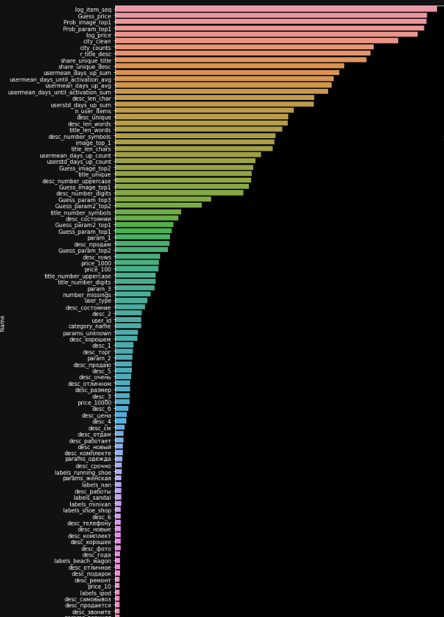
Feature Importance

The lightGBM model performs slightly better than the neural network. However, let’s not discard the neural net because we can stack it with other models.

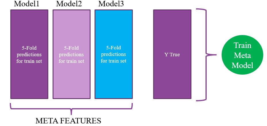
Stacking

A very good introduction to stacking can be found here. In simple terms, the idea is to use multiple models and then make an additional model that learns which one usually perform better. We must avoid target leaking as much as possible so what the way its done is that during a K-Folds cross validation scheme we save the prediction of each fold. You end up with a vector as long as the train set created by your first model. Then you repeat the process a few times for different models. With this stacked data created, you then train a meta model.

Stacking is a method that is criticized for not being practical and something only good for competitions. After all you have to use many different models. However I’d be more careful. First, in some situation where the individual models are small, it is not a problem to use multiple in terms of performance. Second, computing speed is increasing and what currently may look like an ugly mess of neural nets and GBDT may be a standard in the future. After all, a random forest is a mess of trees so maybe in the future we will have model where the base learners are our state of the art models.

The final stack used here is fairly simple:

• 3 lightGBM (different seeds and parameters)
• 1 Catboost
• 1 Neural network

Models files:

• lightGBM script
• catboost script
• Neural Network script

Result

The best single model was lightGBM at 0.2197 and stacking improved the score to 0.2189 (lowest is best). I received a silver medal for the solution being in top 5%. Yay !